The Riemann problem of 1D elastodynamics with Landau's law

Problem statement

Let us consider the system of 1D elastodynamics: $$\begin{equation*} \left\lbrace \begin{array}{l} \displaystyle\frac{\partial\varepsilon}{\partial t} = \frac{\partial v}{\partial x} \, ,\\ \displaystyle\rho_0 \frac{\partial v}{\partial t} = \frac{\partial}{\partial x} \sigma(\varepsilon) \, , \end{array} \right. \end{equation*}$$ where ε denotes the strain, v the particle velocity, and σ the stress. The mass density ρ₀ is assumed to be a constant. Also, we assume that the stress-strain relationship is a polynomial with cubic nonlinearity: $$\begin{equation*} \sigma(\varepsilon) = E\,\varepsilon\, (1 - \beta\,\varepsilon - \delta\,\varepsilon^2) \, . \end{equation*}$$ This constitutive equation is known as Landau's law in the field of nonlinear elasticity. E denotes the Young's modulus, and (β,δ) are dimensionless elastic constants.

We study the Riemann problem, i.e. the case where the initial data is piecewise constant, with one single discontinuity at the abscissa x = x_disc. At t = 0, U_L denotes the left state and U_R the right state: [1,2] $$\begin{equation*} \boldsymbol{U}(x,0) = \left\lbrace \begin{array}{ll} \boldsymbol{U}_L & \text{if } x < x_\textit{disc} \, ,\\ \boldsymbol{U}_R & \text{if } x > x_\textit{disc} \, , \end{array} \right. \end{equation*}$$ where $$\begin{equation*} \boldsymbol{U}(x,t) = \left( \begin{array}{ll} \varepsilon(x,t)\\ v(x,t) \end{array} \right) ,\quad \boldsymbol{U}_L = \left( \begin{array}{ll} \varepsilon_L\\ v_L \end{array} \right) \quad\mbox{and}\quad \boldsymbol{U}_R = \left( \begin{array}{ll} \varepsilon_R\\ v_R \end{array} \right) . \end{equation*}$$

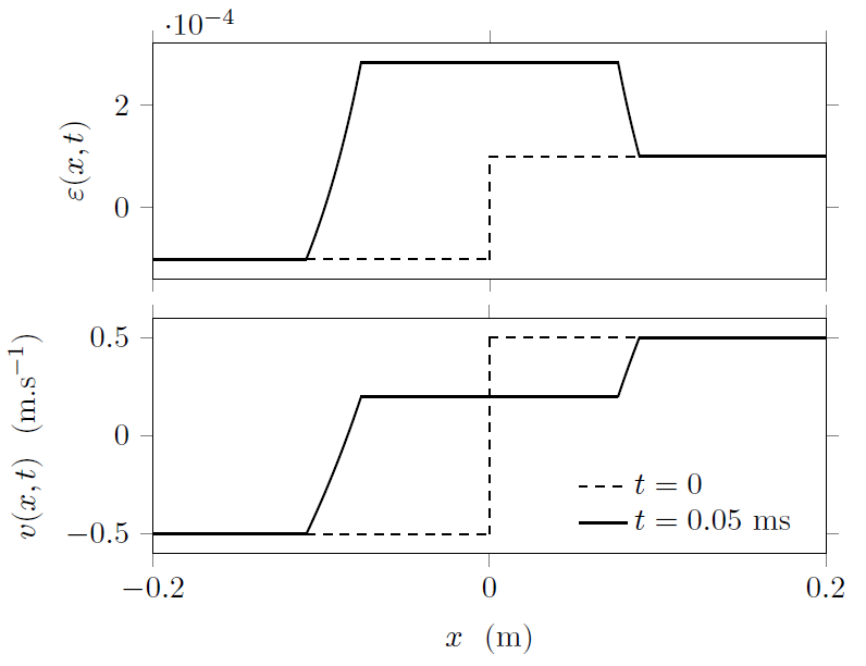
The solution for t > 0 consists of three constant states U_L, U_M and U_R separated by two waves (see figure 1):

• the wave that connects U_L and U_M propagates towards decreasing x and is denoted by the index 1. It can be either a shock S₁, a rarefaction R₁ or a shock-rarefaction SR₁;
• the wave that connects U_M and U_R propagates towards increasing x and is denoted by the index 2. It can be either a shock S₂, a rarefaction R₂ or a rarefaction-shock RS₂.

On figure 1, the configuration corresponds to a case with two rarefactions (R₁R₂).

---

Application

Figure 2 is an interactive tool with which you can predict the nature of the solution to the Riemann problem and compute the intermediate state U_M. In the graphical window, the initial data is represented by the points U_L and U_R. The x-coordinate represents ε×10^-3 and the y-coordinate represents v - v_L (m/s). Therefore, the coordinates of these points are (ε_L×10^-3, 0) and (ε_R×10^-3, v_R - v_L). Dotted lines mark the bounds of the hyperbolicity domain, i.e. the existence domain of the solution. The vertical solid line marks the inflexion point ε₀ = -β/3δ. The nature of the solution, here S₁S₂, is displayed above the graphical window. The curves mark the borders of each region (R₁R₂, R₁S₂, etc.).

Each point can be dragged with the mouse, only horizontally in the case of U_L. The coordinates of a point are displayed when the mouse pointer is over the point. The physical parameters of the material can be set by using the sliders. The first slider sets the linear sound speed $c_0=\sqrt{E/\rho_0}$ . The second and third sliders set the second- and third-order elastic constants respectively. You can compute the intermediate state by clicking the "Solve" button and moving your mouse above U_M. Lastly, you can zoom and move in the ε-v plane by using the navigation bar in the bottom-right corner.

The RiemannElasto1D Toolbox for Matlab generates the analytical solution. To install it, download the files from the following link. Then, follow the instructions in the README file or the help files.

---

References

[1] E. Godlewski and P.A. Raviart: Numerical Approximation of Hyperbolic Systems of Conservation Laws, Springer (1996), ISBN 978-1-4612-0713-9

[2] B. Wendroff: "The Riemann problem for materials with nonconvex equations of state I: Isentropic flow", J. Math. Anal. Appl. 38-2 (1972), 454-466